This article presents a Matlab script to model a Proportional-Integrative-Derivative (PID) controller in which also a disturbance is present. The ode45 Integrator is used to solve the overall dynamic of the extended system.
The scripts
A first file, called pid_function.m contains the call to the ode45 function:
function zdot = pid_function(t,z)

global A B K D d Q R  % import global variables

[K,P] = lqr(A,B,Q,R); % obtain K = [kp kd ki];

%K(1,3)= 0; % This line can be used to cancel the integral term (PID => PD)

u = -K*z;             % obtain the control u

%udot = theta;
%zdot = [xdot; udot];

% Overall dynamic of the extended system
zdot = A*z + B*u + D*d;

end
A second file, called pid_ode.m , is the main script:
%------------------------------
%% clean the workspace

clc           % Clear the console
clear all     % Clear the variables
%close all    % Close all open windows (uncomment to overlap plots among differnt run)

global A B K D d Q R % Create global vars

%------------------------------
%% Define constants

I = 1;
A = [0 1 0; 0 0 0 ; 1 0 0 ];
B = [0;1/I; 0];
D = [0; 1; 0];

q1 = 1;
q2 = 1;
q3 = 1;
r = 1;
Q = [q1 0 0;0 q2 0; 0 0 q3];
R = [r];

%------------------------------
%% Define the integration interval
t_in = 0;              % Initial Time
t_end = 15;            % End Time
tspan = [t_in t_end];  % Time Interval

%------------------------------
%% Define the initial values

d = 10;       % Constant disturbance
x0 = [2 1];   % Position at initial time
u0 = [0];     % Control vector at initial time
z0 = [x0'; u0'];

%------------------------------
%% Call the ode

% Define a boolean variable to debug the ode on zdot
enable_ode = 1;
if enable_ode

  options = odeset('abstol',1e-10,'reltol',1e-5);   % Define tollerances
  [t,z]   = ode45('pid_function',tspan,z0,options); % Call the ode

  % Compute the control vector u
  for i=1:length(t)
    % u=-K*x
    u(i,:)=-K*(z(i,1:3))';
  end

end

% Define a boolean variable to print (or not) figures
enable_figure=1;
if enable_figure

  figure(1);

  % define figure parameters
    set(1, 'NextPlot', 'add')
    set(1,'Units', 'normalized')
    set(1,'Position', [.2 0 0.6 0.8])
    set(1,'NumberTitle', 'off')
    set(1,'Name', 'Angular position and velocity, control and errors')

% Subplot of Angular Position
  subplot(3,1,1);
    plot(t,z(:,1))
    % hold all % uncomment to overlap plots among differnt run
    grid on
    xlabel('Time','fontsize',8,'fontname','tahoma','fontweight','bold')
    ylabel('Angular position','fontsize',8,'fontname','tahoma','fontweight','bold')

% Subplot of Angular Velocity
  subplot(3,1,2);
    plot(t,z(:,2))
    % hold all % uncomment to overlap plots among differnt run
    grid on
    xlabel('Time','fontsize',8,'fontname','tahoma','fontweight','bold')
    ylabel('Angular Velocity','fontsize',8,'fontname','tahoma','fontweight','bold')

% Subplot of the control vector u
  subplot(3,1,3);
    plot(t,u)
    % hold all % uncomment to overlap plots among differnt run
    grid on
    xlabel('Time','fontsize',8,'fontname','tahoma','fontweight','bold')
    ylabel('Control Vector','fontsize',8,'fontname','tahoma','fontweight','bold')

end

% Print K: "K= [ 2.4142 ; 2.4142 ; 1.0000 ]"
fprintf('K = [ %f ; %f ; %f ]', K(1), K(3), K(3))
disp('End of script.')
Results
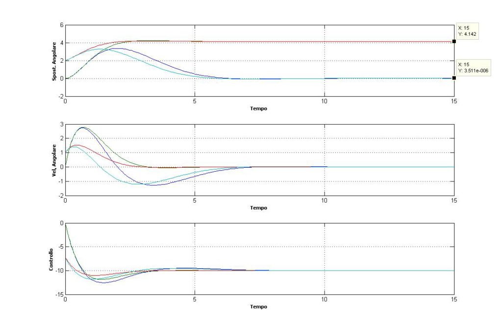
Four different cases were run, with both a PD (Partial-Derivative) and a PID system, and two different initial positions:
- Purple lines : PID, x0=[0,0]
- Cyan lines: PID, x0=[2,1]
- Red lines : PD, x0=[2,1]
- Green lines: PD, x0=[0,0]
K = 2.4142 2.4142 1.0000
From the top: Angular position, angular velocity and value of the control vector as a function of time.
Discussion and Conclusion
As highlighted in the first sub-plot of the previous figure, the angular position of the PID system – after the initial transient – is zero (purple and cyan lines). Conversely in a PD system, where there is no integral term, red and green lines, there is a residual angle theta_end= 4.142 = D/Kp (the PD system was obtained setting the third parameter of K equal to zero in the 7th line of pid_function.m). The results do not change when changing the initial conditions on the position.

